README

The package bayesRecon implements several methods for probabilistic reconciliation of hierarchical time series forecasts.

News

:boom: [2024-05-29] Added reconc_MixCond and reconc_TDcond and the vignette “Reconciliation of M5 hierarchy with mixed-type forecasts”.

:boom: [2023-12-19] Added the vignette “Properties of the reconciled distribution via conditioning”.

:boom: [2023-08-23] Added the vignette “Probabilistic Reconciliation via Conditioning with bayesRecon”. Added the schaferStrimmer_cov function.

Installation

install.packages("bayesRecon", dependencies = TRUE)

# install.packages("devtools")
devtools::install_github("IDSIA/bayesRecon", build_vignettes = TRUE, dependencies = TRUE)

Usage

The package bayesRecon implements functions for probabilistic forecast reconciliation. In the following examples, we show how to use the main reconciliation functions of the package for different types of base forecasts.

Example 1: Gaussian forecast distributions

Let us consider a hierarchy with 4 bottom time series and 3 upper time series, as shown in the figure above. The hierarchy is specified by the aggregation matrix A:

A <- matrix(c(
  1, 1, 1, 1,
  1, 1, 0, 0,
  0, 0, 1, 1
), nrow = 3, byrow = TRUE)

In this example, we assume that the base forecasts are multivariate Gaussian, which is a common choice for real-valued time series.

To generate the hierarchical time series, we first randomly simulate the bottom series using an AR(1) process and then aggregate them using A to obtain the upper series.

set.seed(1234)

# Simulate bottom series from AR(1) processes
n_obs <- 12  # length of the time series
B_ts <- matrix(nrow = 4, ncol = n_obs)
for (j in 1:4) {
  B_ts[j, ] <- arima.sim(model = list(ar = 0.8), n = n_obs, sd = 0.5)
}
# Aggregate to obtain upper series 
U_ts <- A %*% B_ts
# Convert to mts
B_ts <- ts(t(B_ts))
U_ts <- ts(t(U_ts))
Y_ts <- cbind(U_ts, B_ts)

We compute the base forecasts using an ETS model with Gaussian predictive distribution, implemented in the forecast package. For simplicity, we only compute one-step-ahead forecasts, but the same procedure can be applied to multi-step-ahead forecasts.

We also save the in-sample residuals of the fitted models, as we later need them to estimate the covariance matrix of the base forecasts.

library(forecast)

base_fc_mean <- c()
residuals <- matrix(nrow = n_obs, ncol = ncol(Y_ts))
for (j in 1:ncol(Y_ts)) {
  fit <- forecast::ets(Y_ts[,j], additive.only = TRUE)  # fit ets on each time series
  base_fc_mean[j] <- as.numeric(forecast::forecast(fit, h = 1)$mean)
  residuals[,j] <- fit$residuals
}

We then analytically compute the reconciled forecasts via conditioning using the reconc_gaussian and the reconc_t functions. The reconciled forecasts produced by reconc_gaussian are multivariate Gaussian, and they are equivalent to MinT reconciliation (Zambon et al. 2024). The reconc_t method adopts a Bayesian approach to account for the uncertainty of the covariance matrix of the base forecasts; the reconciled forecasts, which are multivariate Student-t, are typically better calibrated (see Carrara et al. 2025 for details).

library(bayesRecon)

# Reconcile with both methods
rec_g <- reconc_gaussian(
  A,
  base_fc_mean,
  residuals = residuals,
  return_upper = TRUE
)
rec_t <- reconc_t(
  A,
  base_fc_mean,
  y_train = Y_ts,
  residuals = residuals,
  return_upper = TRUE
)

# Compare means of the base and reconciled forecasts
means <- rbind(c(base_fc_mean),
               c(rec_g$upper_rec_mean, rec_g$bottom_rec_mean),
               c(rec_t$upper_rec_mean, rec_t$bottom_rec_mean))
rownames(means) <- c("base", "reconc_gaussian", "reconc_t")
colnames(means) <- c("T", "A", "B", "AA", "AB", "BA", "BB")
print(round(means, 2))
#>                     T     A     B    AA    AB    BA    BB
#> base            -2.64 -2.24 -0.35 -2.06 -0.18 -0.19 -0.47
#> reconc_gaussian -2.73 -2.25 -0.49 -2.05 -0.20 -0.14 -0.35
#> reconc_t        -2.87 -2.37 -0.50 -2.02 -0.35 -0.11 -0.39

Finally, we compare the reconciled forecast distributions for the top series T obtained with the two methods by plotting their marginal densities.

Example 2: discrete forecast distributions

We consider the same hierarchy of Example 1; however, we assume that the base forecasts are Poisson distributions, which is a common choice for count time series.

We randomly generate the bottom series using Poisson distributions with time-varying rates that include a monthly seasonal pattern; we then aggregate them using A to obtain the upper series.

set.seed(123)
n_obs <- 60

# Bottom time series are obtained by drawing from Poisson distributions with time-varying rates
lambda_bls <- c(3, 4, 5, 6)  # baseline Poisson rates for bottom series
seas <- 1.5*sin(2*pi*(1:n_obs)/12)  # specify monthly seasonality (period = 12) 
lambdas <- outer(lambda_bls, seas, FUN = "+")  # adds seasonality to each baseline (4 x n_obs matrix)
lambdas <- lambdas + matrix(rnorm(4 * n_obs, sd = 0.1), nrow = 4) # add small Gaussian noise to rates

# Simulate bottom-level count time series
B_ts <- matrix(rpois(4 * n_obs, lambdas), nrow = 4)
# Aggregate to obtain upper series
U_ts <- A %*% B_ts
# Convert to mts
B_ts <- ts(t(B_ts), frequency = 12)
U_ts <- ts(t(U_ts), frequency = 12)
Y_ts <- cbind(U_ts, B_ts)

We compute the one-step-ahead base forecasts using the package glarma, which is specific for count time series. We forecast using a glarma model with Poisson predictive distribution.

library(glarma)

base_fc <- list()
for (j in 1:ncol(Y_ts)) {
  yj <- Y_ts[,j]  # time series j
  X <- matrix(c(rep(1, length(yj)), seas), ncol = 2)  # matrix of exogenous regressors
  X_new <- matrix(c(1, 1.5*sin(2*pi*(n_obs + 1)/12)), ncol = 2)  # regressors for the forecast period
  fit <- glarma::glarma(yj, X, type = "Poi")  # fit the model
  # Compute base forecasts, which are Poisson distributions specified by the rate parameter 
  fc_lambda <- glarma::forecast(fit, newdata = X_new, n.ahead = 1)$mu  
  # Save the base forecast parameters in a list of lists, one for each series
  base_fc[[j]] <- list(lambda = fc_lambda)  
}

We then compute the reconciled forecasts using the bottom-up importance sampling (BUIS) algorithm (see Zambon et al. 2024 for details). The output of reconc_BUIS is a joint sample from the reconciled distribution, which can be used to compute any desired summary (e.g. mean, quantiles, etc.).

rec_buis <- reconc_BUIS(
  A,
  base_fc,
  in_type = "params",
  distr = "poisson",
  num_samples = 20000
)
samples_buis <- rbind(rec_buis$upper_rec_samples,
                      rec_buis$bottom_rec_samples)
rownames(samples_buis) <- c("T", "A", "B", "AA", "AB", "BA", "BB")

# Compute reconciled means
print(round(rowMeans(samples_buis), 2))
#>     T     A     B    AA    AB    BA    BB 
#> 20.69  8.36 12.33  4.05  4.31  5.83  6.50

# Compute upper quantiles of the reconciled forecast distributions:
print(apply(samples_buis, 1, quantile, probs = c(0.80, 0.95)))
#>      T  A  B AA AB BA BB
#> 80% 23 10 14  5  6  8  8
#> 95% 26 12 16  7  7  9 10

Finally, we compare the base and reconciled forecasts for the top series T by plotting the base and reconciled forecast distributions.

Similar results can be obtained with reconc_MCMC, which is a bare-bones implementation of the Metropolis-Hastings algorithm. However, we recommend using reconc_BUIS rather than reconc_MCMC for reconciling discrete forecasts.

Example 3: mixed-type forecast distributions

In many large hierarchies the bottom series are low-count integers (e.g., item-level sales), while the upper series can be considered as real-valued due to the smoothing effect of aggregation (e.g., total sales). These hierarchies are often referred to as mixed, since forecasts for the bottom series are discrete distributions, while forecasts for the upper series are continuous distributions. The functions reconc_MixCond and reconc_TDcond handle this mixed case: they take a list of discrete distributions for the bottom level and a multivariate Gaussian for the upper levels. These functions implement different methods for reconciling mixed hierarchies; we recommend using reconc_MixCond for moderately sized hierarchies and reconc_TDcond for large hierarchies (see Zambon et al. 2024 for details).

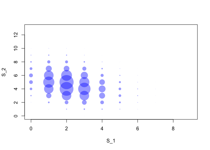
Let us consider a hierarchy with 3 upper series and 52 bottom series arranged in 2 groups of 26:

We randomly generate the bottom count time series as in Ex. 2; we then aggregate them using A to obtain the upper series.

set.seed(12)
n_b   <- 52   # number of bottom series 
n_u   <- 3    # number of upper series
n_obs <- 60   # series length

# Build aggregation matrix A for the hierarchy in the figure above
A <- rbind(rep(1, n_b),
           c(rep(1, 26), rep(0, 26)),
           c(rep(0, 26), rep(1, 26)))

# Assume Poisson data generating process + monthly seasonality
lambda_levels <- runif(n_b, min = 0.1, max = 2)
seas <- 1 + .5*sin(2*pi*(1:n_obs)/12)
lambdas <- outer(lambda_levels, seas, FUN = "*")

# Generate bottom series
B_ts <- matrix(rpois(n_obs * n_b, lambdas), nrow = n_b)
# Aggregate to obtain upper series
U_ts <- A %*% B_ts
# Convert to mts
B_ts <- ts(t(B_ts), frequency = 12)
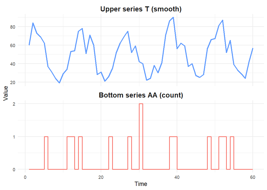
U_ts <- ts(t(U_ts), frequency = 12)

We show a comparison of upper and bottom time series. Even though the bottom series are made of low counts, the upper series can be considered as real-valued due to the smoothing effect of aggregation.

We compute the one-step-ahead base forecasts for each upper series with an additive ETS model, implemented in the forecast package. We use the covariance matrix of the in-sample residuals, estimated via shrinkage using the schaferStrimmer_cov function, as the joint forecast covariance of the upper series.

mu_u <- numeric(n_u)
residuals_u <- matrix(nrow = n_obs, ncol = n_u)
for (j in seq_len(n_u)) {
  fit <- forecast::ets(ts(U_ts[, j]), additive.only = TRUE)
  mu_u[j] <- as.numeric(forecast::forecast(fit, h = 1)$mean)
  residuals_u[, j] <- fit$residuals
}
# Estimate the covariance matrix via Schafer-Strimmer shrinkage from in-sample residuals
Sigma_u <- bayesRecon::schaferStrimmer_cov(residuals_u)$shrink_cov 
# Save upper base forecasts as a list with mean and covariance
base_fc_upper <- list(mean = mu_u, cov = Sigma_u)

We compute the one-step-ahead base forecasts for the bottom series using the package glarma. The base forecasts are Poisson distributions.

base_fc_bottom <- list()
for (j in seq_len(n_b)) {
  bj <- B_ts[,j]
  X <- matrix(c(rep(1, length(bj)), seas), ncol = 2)  # matrix of exogenous regressors
  X_new <- matrix(c(1, 1 + .5*sin(2*pi*(n_obs + 1)/12)), ncol = 2)  # regressors for the forecast period
  fit <- glarma(bj, X, type = "Poi")
  # Bottom base forecasts are Poisson distributions, specified by the rate parameter 
  fc_lambda <- glarma::forecast(fit, newdata = X_new, n.ahead = 1)$mu
  # Save the parameters of bottom base forecasts in a list of lists, one for each series
  base_fc_bottom[[j]] <- list(lambda = fc_lambda)
}

We reconcile using both reconc_MixCond (importance-sampling based conditioning) and reconc_TDcond (top-down conditioning). These functions implement different methods for reconciling mixed hierarchies, but they share the same input arguments and output structure.

res_mc <- reconc_MixCond(
  A, base_fc_bottom, base_fc_upper,
  bottom_in_type = "params", distr = "poisson",
  num_samples = 2e4, 
  return_type = "pmf"
)

res_td <- reconc_TDcond(
  A, base_fc_bottom, base_fc_upper,
  bottom_in_type = "params", distr = "poisson",
  num_samples = 2e4, 
  return_type = "pmf"
)

The joint forecast distribution can be obtained by specifying return_type = "samples". In this case, since we set return_type = "pmf", the functions return the reconciled marginal forecast distributions as probability mass functions (PMFs). From these PMFs, we can compute any desired summary (e.g. mean, quantiles, etc.) using the PMF functions.

# Compare the upper means of the base and reconciled forecasts
upper_means <- rbind(
  base    = mu_u,
  MixCond = sapply(res_mc$upper_rec_pmf, PMF_get_mean),
  TDcond  = sapply(res_td$upper_rec_pmf, PMF_get_mean)
)
colnames(upper_means) <- c("T", "A", "B")
print(round(upper_means, 2))
#>             T     A     B
#> base    56.98 19.84 34.31
#> MixCond 59.24 23.55 35.68
#> TDcond  55.99 20.42 35.57

# Compare the 95% upper quantiles of the base and reconciled forecast distributions
upper_q <- rbind(
  base    = sapply(mu_u, function(m) qnorm(0.95, mean = m, sd = sqrt(Sigma_u[1,1]))),
  MixCond = sapply(res_mc$upper_rec_pmf, PMF_get_quantile, p = 0.95),
  TDcond  = sapply(res_td$upper_rec_pmf, PMF_get_quantile, p = 0.95)
)
colnames(upper_q) <- c("T", "A", "B")
print(round(upper_q, 2))
#>             T    A     B
#> base    81.93 44.8 59.26
#> MixCond 71.00 30.0 44.00
#> TDcond  81.00 34.0 51.00

Finally, we compare the base forecast and the two reconciled forecast distributions for the top series T. The base distribution is a Gaussian density (line); the reconciled distributions are discrete PMFs (bars). The black triangle indicates the actual value of T. We refer to Zambon et al. 2024 for a detailed comparison of the two methods for reconciling mixed hierarchies of different sizes.

References

Carrara, C., Corani, G., Azzimonti, D., Zambon, L. (2025). Modeling the uncertainty on the covariance matrix for probabilistic forecast reconciliation. arXiv preprint arXiv:2506.19554. Available here

Corani, G., Azzimonti, D., Augusto, J.P.S.C., Zaffalon, M. (2021). Probabilistic Reconciliation of Hierarchical Forecast via Bayes’ Rule. ECML PKDD 2020. Lecture Notes in Computer Science, vol 12459. DOI

Corani, G., Azzimonti, D., Rubattu, N. (2024). Probabilistic reconciliation of count time series. International Journal of Forecasting 40 (2), 457-469. DOI

Zambon, L., Azzimonti, D. & Corani, G. (2024). Efficient probabilistic reconciliation of forecasts for real-valued and count time series. Statistics and Computing 34 (1), 21. DOI

Zambon, L., Agosto, A., Giudici, P., Corani, G. (2024). Properties of the reconciled distributions for Gaussian and count forecasts. International Journal of Forecasting 40 (4), 1438-1448. DOI

Zambon, L., Azzimonti, D., Rubattu, N., Corani, G. (2024). Probabilistic reconciliation of mixed-type hierarchical time series. Proceedings of the Fortieth Conference on Uncertainty in Artificial Intelligence, in Proceedings of Machine Learning Research 244:4078-4095. Available here.

Contributors

Getting help

If you encounter a clear bug, please file a minimal reproducible example on GitHub.

bayesRecon: BAyesian reCONciliation of hierarchical forecasts