trendseries: extract trends from time series

trendseries provides a unified interface to extract trends, cycles, and seasonal components from time series. Most filtering methods in R are designed for ts objects, but datasets typically come in a data.frame format with a date column, which makes applying filters cumbersome. trendseries bridges this gap: augment_trends(), decompose_series(), deseason_series(), and detrend_series() all work directly on data.frame/tibble objects, while extract_trends() provides the same methods for ts/xts/zoo objects when you need to stay in native time-series format.

Installation

trendseries is available on CRAN

install.packages("trendseries")

You can install the development version of trendseries from GitHub.

# install.packages("remotes")
remotes::install_github("viniciusoike/trendseries")

Main Functions

The package provides four main functions for data.frame/tibble/data.table workflows:

• augment_trends(): adds trend columns to the original dataset.
• decompose_series(): splits a series into trend, seasonal, and remainder components.
• deseason_series(): wraps decompose_series() to return a seasonally adjusted series.
• detrend_series(): wraps augment_trends() to return the deviation from trend (the cycle).

Each has a ts/xts/zoo-native counterpart via extract_trends(), for workflows that stay in native time-series format.

Usage

Time series have a specific structure in R (ts) and most filtering methods are designed for ts objects. However, datasets typically come in a data.frame format with a date column, which can make applying filters cumbersome.

trendseries aims to make this process easy and flexible. The example below computes three filters (HP, STL, and moving average) on a quarterly index of construction activity. Note that the augment_trends() function automatically detects the frequency of the data and uses conventional defaults for the HP filter.

library(trendseries)
library(ggplot2)
data(gdp_construction)
# Computes multiple trends at once
series <- gdp_construction |>
  # Automatically detects frequency
  # Trends are added as new columns to the original dataset
  augment_trends(
    value_col = "index",
    methods = c("hp", "stl", "ma")
  )
#> Auto-detected quarterly (4 obs/year)
#> Computing HP filter (two-sided) with lambda = 1600
#> Computing STL trend with s.window = periodic
#> Computing 2x4-period MA (auto-adjusted for even-window centering)

series
#> # A tibble: 124 × 5
#>    date       index trend_hp trend_stl trend_ma
#>    <date>     <dbl>    <dbl>     <dbl>    <dbl>
#>  1 1995-01-01 100       101.     102.      NA  
#>  2 1995-04-01 100       101.     101.      99.7
#>  3 1995-07-01 100       102.     100.      99.6
#>  4 1995-10-01 100       103.      99.4    101. 
#>  5 1996-01-01  97.8     103.     101.     102. 
#>  6 1996-04-01 101.      104.     102.     103. 
#>  7 1996-07-01 107.      104.     103.     104. 
#>  8 1996-10-01 103.      105.     104.     106. 
#>  9 1997-01-01 101.      106.     106.     109. 
#> 10 1997-04-01 108.      106.     109.     111. 
#> # ℹ 114 more rows

An equivalent extract_trends() function is also available for ts objects.

stl_trend <- extract_trends(AirPassengers, methods = "stl")
#> Computing STL trend with s.window = periodic
plot.ts(AirPassengers)
lines(stl_trend, col = "#C53030")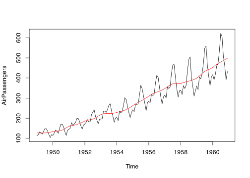

Available Methods

trendseries supports 20 trend estimation methods, covering the most commonly used approaches in econometrics and statistics. The Trend Extraction Methods vignette describes each one — when to use it and which parameters it takes.

Decomposition

To split a series into trend, seasonal, and remainder components, use decompose_series(). It supports STL, regression, classical moving-average, Basic Structural Model (BSM), and X-13ARIMA-SEATS decomposition:

gdp_construction |>
  decompose_series(value_col = "index", methods = "stl")

See the Decomposing Series vignette for details.

Learn More

See the vignettes for detailed examples and usage patterns:

• Introduction to trendseries

• Augmenting Trends

• Trend Extraction Methods

• Moving Averages

• Econometric Filters

• Decomposing Series

• Detrending Series